
Summary:
- This project is to train model to steer the simulation vehicle to be on the right track. The input to the model measurement is steering angle collected from the pre-run. The vehicle image corresponding to the certain steering angle is stored at the pre-run as well.Then, the stored images are used to train the model so the angle will be anticipated when a image is collected while the vehicle is driving at actual run.
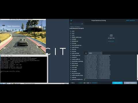
Final result (please click the below thumbnail to play a video):
Behavioral Cloning Project
The goals / steps of this project are the following:
- Use the simulator to collect data of good driving behavior (steering angle, image)
- read data and pre-processing
- Build, a convolution neural network in Keras that predicts steering angles from images
- Train and validate the model with a training and validation set
- Test that the model successfully drives around track one without leaving the road
- Summarize the results with a written report
- Things to consider: rubric points
Overview
- Required files to run simulation:
My project includes the following files:
- model_r0.py containing the script to create and train the model
- drive.py for driving the car in autonomous mode
- model.h5 containing a trained convolution neural network
- README.md summarizing the results
- run4.mp4 video clip on autonomous mode
- How to run simulation
Using the Udacity provided simulator and my drive.py file, the car can be driven autonomously around the track by executing
python drive.py model.h5 run4
- Code overview
The model_r0.py file contains the code for training and saving the Convolution Neural Network (CNN).
The file shows the pipeline I used for training and validating the model as well as comments to explain how the code works.
- Model Architecture and Training Strategy
a. Model arhicture overview
- My model consists of a Convolution Neural Network (CNN) with 5x5 filter sizes and depths between 24,36,48,64,64.
The model includes ReLU (Rectified Linear Unit) layers to introduce nonlinearity.
model.add(Conv2D(24,(5,5),strides=(2,2),activation="relu"))
model.add(Conv2D(36,(5,5),strides=(2,2),activation="relu"))
model.add(Conv2D(48,(5,5),strides=(2,2),activation="relu"))

model.add(Conv2D(64,(3,3),activation="relu"))
model.add(Conv2D(64,(3,3),activation="relu"))
- The data is normalized in the model using a Keras lambda layer.
model.add(Lambda(lambda x: x/127.5 - 1.,
        input_shape=(row, col, ch),
        output_shape=(row, col, ch)))
- CNN network uses flatten, then engage 3 fully engaged layers (100/50/10).
model.add(Flatten())


model.add(Dense(100))

model.add(Dropout(0.2)) # overfitting
model.add(Dense(50))

model.add(Dropout(0.2)) # overfitting
model.add(Dense(10))

model.add(Dropout(0.2)) # overfitting
model.add(Dense(1))
b. Beat overfitting…
- The model contains dropout layers in order to reduce overfitting.
model.add(Dropout(0.2)) # overfitting
- The model was trained and validated by different data sets to ensure that the model was not overfitting.
batch_size=32
# compile and train the model using the generator function
train_generator = generator(train_samples, batch_size=batch_size)
validation_generator = generator(validation_samples, batch_size=batch_size)

- The model was tested by running it through the simulator. The passing criteria is that the vehicle could stay on the track.
c. Model parameter tuning
- The model used an adam optimizer, so the learning rate was not tuned manually.
model.compile(loss='mse',optimizer='adam')
d. Appropriate training data
Training data (combining both sample data given by Udacity and my own driving data set) was chosen to keep the vehicle driving on the road. I used a combination of center lane driving, recovering from the left and right sides of the road which is part of my own driving data set.
For details about how I created the training data, see the next section.
Detailed overview
a. Solution Design Approach
The overall strategy for deriving a model architecture takes an idea from Nvidia’s approachNvidia paper
The reason why this model architecture was chosen is it’s already a proven working solution(then, why not give a go?).
In order to gauge how well the model was working, I split my image and steering angle data into a training and validation set. I found that my first model had a low mean squared error on the training set but a high mean squared error on the validation set. This implied that the model was overfitting.

To combat the overfitting, I modified the model so that “drop out” strategy was applied:
model.add(Dropout(0.2)) # overfitting
Then the overfitting was improved.
The final step was to run the simulator to see how well the car was driving around track one.
At the end of the process, the vehicle is able to drive autonomously around the track without leaving the road.
b. Final Model Architecture
The final model architecture are shown here:
model = Sequential()
model.add(Lambda(lambda x: x/127.5 - 1.,
        input_shape=(row, col, ch),
        output_shape=(row, col, ch)))
model.add(Cropping2D(cropping=((70,25),(0,0))))
#model.add(BatchNormalization()) # overfitting
model.add(Conv2D(24,(5,5),strides=(2,2),activation="relu"))
#model.add(Conv2D(24,(5,5),strides=(2,2),activation="relu"))
#model.add(BatchNormalization()) # overfitting
model.add(Conv2D(36,(5,5),strides=(2,2),activation="relu"))
#model.add(BatchNormalization()) # overfitting
model.add(Conv2D(48,(5,5),strides=(2,2),activation="relu"))
#model.add(BatchNormalization()) # overfitting
model.add(Conv2D(64,(3,3),activation="relu"))
model.add(Conv2D(64,(3,3),activation="relu"))

model.add(Flatten())

model.add(Dense(100))
model.add(Dropout(0.2)) # overfitting
model.add(Dense(50))
model.add(Dropout(0.2)) # overfitting
model.add(Dense(10))
model.add(Dropout(0.2)) # overfitting
model.add(Dense(1))
#model.add(Dense(120))
#model.add(Dense(84))
#model.add(Dense(1))

model.compile(loss='mse',optimizer='adam')
#model.fit(X_train,y_train,validation_split = 0.2,shuffle=True,epochs = 2)
history_object = model.fit_generator(train_generator, \
            steps_per_epoch=math.ceil(len(train_samples)/batch_size), \
            validation_data=validation_generator, \
            validation_steps=math.ceil(len(validation_samples)/batch_size), \
            epochs=5, verbose=1)
model.save('model.h5')
c. Creation of the Training Set & Training Process
To capture good driving behavior, I first recorded two laps on track one using center lane driving. Here is an example image of center lane driving:


Then I repeated this process on track two in order to get more data points.
To augment the data sat, flipped images was used. For example, here is the code for flip image augmentation:
            augmented_images,augmented_measurements = [],[]
            for image, measurement in zip(images,measurements):
                augmented_images.append(image)
                augmented_measurements.append(measurement)
                augmented_images.append(cv2.flip(image,1))
                augmented_measurements.append(measurement*-1.0)
I finally randomly shuffled the data set and put 20% of the data into a validation set.
from sklearn.model_selection import train_test_split
train_samples, validation_samples = train_test_split(samples, test_size=0.2)
I used this training data for training the model. The validation set helped determine if the model was over or under fitting. The ideal number of epochs was 5 as evidenced by following experimental trials. I used an adam optimizer so that manually training the learning rate wasn’t necessary.


d. Here is the final result of video record during autonomous mode driving:
- Could try different modeling architectural strategy.
- things to try